
Efron’s partial likelihood estimator is a method to handle tied events in Cox Survival Regression. Here we implement the method in TensorFlow to use it as an objective in a computational graph.
Cox Proportional Hazards Recap
In Survival Analysis each observation can be expressed as a triple , where is a set of covariates, is the follow-up time, and is the binary event indicator or censoring status. Cox Proportional Hazards model is probably one of the most popular methods to model time-to-event data. The model estimates the risk or probability of any arbitrary event of interest to occur at time t given that the individual has survived until that time. This is called a hazard function and in the Cox framework is expressed like this:
Here the first term is called the baseline hazard and depends only on time. The baseline hazard remains unspecified, thus no particular distribution of survival times is assumed in the model. This is one of the reasons for the Cox model being so popular. The second term depends only on the covariates, but not time. This implies the proportional hazard assumption, i.e. the effects of covariates on survival are constant over time.
Estimation of the Cox Model
The full maximum likelihood requires that we specify the baseline hazard . In 1972 Sir David Cox explained how to avoid having to specify this component explicitly and proposed a partial likelihood that depends only on the parameters of interest, but not time:
Here - predicted risk for individual . This function iterates over subjects who fail and takes into account censored observations only in the risk set (denominator). The problem with this likelihood is that it works only for continuous time survival data, which is obviously not the case in practical applications where multiple events may occur at the same (discrete) time. This complicates things a bit.
Handling ties with Efron Approximation
A number of approaches have been suggested to handle tied events including the exact method that basically considers all possible orders of events that occurred at the same time. The exact approach, however, becomes computationally intensive as the number of ties grows. More efficient approaches have been proposed by Breslow and Efron. Efron’s method though is considered to give better approximation to the original partial likelihood and is the default for R survival package:
Here is a set of individuals that failed at time .
An example
To understand what is going on here, let’s consider an example. Say we observe a population with the following lifetimes and some risk value predicted for each individual:
observed_times = np.array([5,1,3,7,2,5,4,1,1])
censoring      = np.array([1,1,0,1,1,1,1,0,1])
predicted_risk = np.array([0.1,0.4,-0.2,0.2,-0.3,0.0,-0.1,0.3,-0.4])
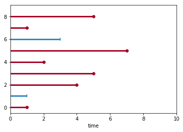
So these are 9 observations whit red lines indicating the lifespan of individuals who experienced and event () and blue lines denote right-censored () cases. Here we have ties at and .
As we typically like to optimize the logarithm of the likelihood function, let’s rewrite Efron’s formula again and give names to the key terms:
Using our toy dataset we can break down the equation into pieces and construct a table [first loop]. Note that the table is sorted by observed lifespans.
| 5 | 7 | 1 | 0.2 | 0.2 | 1.22 | 1.22 |
| 4 | 5 | 1 | 0.1 | 0.1 | 2.105 | 2.33 |
| 5 | 1 | 0.0 | 3.33 | |||
| 3 | 4 | 1 | -0.1 | -0.1 | 0.905 |
4.23 |
| 3 | 0 | -0.2 | 5.05 | |||
| 2 | 2 | 1 | -0.3 | -0.3 | 0.741 | 5.79 |
| 1 | 1 | 1 | 0.4 | 0 | 2.162 | 7.28 |
| 1 | 0 | 0.3 | 8.63 | |||
| 1 | 1 | -0.4 | 9.30 | |||
| failure times | observed lifespans | censoring | predicted risk | tie_risk | tie_hazard | cum_sum / cum_hazard |
Now we just need to put the values together [second loop] :
Implementation
We are going to store intermediate results in the following tensorflow variables:
tie_count   = tf.Variable([], dtype=tf.uint8,   trainable=False)
tie_risk    = tf.Variable([], dtype=tf.float32, trainable=False)
tie_hazard  = tf.Variable([], dtype=tf.float32, trainable=False)
cum_hazard  = tf.Variable([], dtype=tf.float32, trainable=False)
These arrays are gathered while looping over individual failure times for the first time. Before we actually do the looping, we need to:
1). order the observation according to the observed lifespans:
def efron_estimator_tf(time, censoring, prediction):
    n        = tf.shape(time)[0]
    sort_idx = tf.nn.top_k(time, k=n, sorted=True).indices
    risk     = tf.gather(prediction, sort_idx)
    events   = tf.gather(censoring, sort_idx)
    otimes   = tf.gather(time, sort_idx)
2). obtain unique failure times such that :
otimes_cens   = otimes * events
unique_ftimes = tf.boolean_mask(otimes_cens, tf.greater(otimes_cens,0))
unique_ftimes = tf.unique(unique_ftimes).y
m = tf.shape(unique_ftimes)[0] # number of unique failure times
Now we are ready for looping. Indexing is the only part the might seem tricky because of type conversions. The code below is one step of the loop. First, we count number ties for each failure time:
idx_b = tf.logical_and(
    tf.equal(otimes, unique_ftimes[i]),
    tf.equal(events, tf.ones_like(events)) )

tie_count = tf.concat([tie_count, [tf.reduce_sum(tf.cast(idx_b, tf.uint8))]], 0)
Since tie_risk and tie_hazard ignore censored observations they can be gathered as follows:
idx_i = tf.cast(
    tf.boolean_mask(
        tf.lin_space(0., tf.cast(n-1,tf.float32), n),
        tf.greater(tf.cast(idx_b, tf.int32),0)
    ), tf.int32 )

tie_risk   = tf.concat([tie_risk, [tf.reduce_sum(tf.gather(risk, idx_i))]], 0)
tie_hazard = tf.concat([tie_hazard, [tf.reduce_sum(tf.gather(tf.exp(risk), idx_i))]], 0)
Finally, cum_hazard takes into account censored observations, so indexing changes:
# this line actually stays outside of the loop
cs = tf.cumsum(tf.exp(risk))

idx_i = tf.cast(
    tf.boolean_mask(
        tf.lin_space(0., tf.cast(n-1,tf.float32), n),
        tf.greater(tf.cast(tf.equal(otimes, unique_ftimes[i]), tf.int32),0)
    ), tf.int32 )

cum_hazard = tf.concat([cum_hazard, [tf.reduce_max(tf.gather( cs, idx_i))]], 0)
Once these four vectors are gathered we will have to make the while loop again to finally calculate the likelihood:
def loop_2_step(i, tc, tr, th, ch, likelihood):
    l = tf.cast(tc[i], tf.float32)
    J = tf.lin_space(0., l-1, tf.cast(l,tf.int32)) / l
    Dm = ch[i] - J * th[i]
    likelihood = likelihood + tr[i] - tf.reduce_sum(tf.log(Dm))
    return i + 1, tc, tr, th, ch, likelihood

loop_2_out = tf.while_loop(
    loop_cond, loop_2_step,
    loop_vars = [i, tie_count, tie_risk, tie_hazard, cum_hazard, log_lik],
    shape_invariants = [i.get_shape(),tf.TensorShape([None]),tf.TensorShape([None]),tf.TensorShape([None]),tf.TensorShape([None]),log_lik.get_shape()]
)

log_lik = loop_2_out[-1]
Complete TensorFlow code for the function is on GitHub. If you run it on our dummy data you get 9.8594456.
If you find mistakes or have suggestions how to optimize the code, I would be happy if you share those with me!
Validation with R and Lifelines
Here is a script that validates the TensorFlow code with Efron implementations from Lifelines (thanks to Cameron) and R-survival package.